Basic Example
This section gives an example of a basic usage case of the Frankford package. It is assumed that the user is familiar with the Levenberg-Marquardt algorithm and the numpy python package.
In this section, we will fit a set of Gaussian curves to generated data. We will fit 200 curves of 100 points each.
Import
Import the needed modules.
>>> import numpy as np
>>> import math
>>> import frankford
Prepare Data
Set constants.
>>> CURVE_COUNT = 200
>>> POINT_COUNT = 100
Use evenly spaced values of the independent variable x from -100 to +100.
>>> x_data = np.linspace(start=-100.0, stop=100.0, num=POINT_COUNT, dtype=np.double)
Use the point_dtype d-type to store values and uncertainties of the data to be fitted.
>>> noise = 1.0
>>> rng = np.random.default_rng(0)
>>> y_data = np.empty((POINT_COUNT, CURVE_COUNT), dtype=frankford.point_dtype)
>>> for i in range(CURVE_COUNT):
...     amp = rng.uniform(low=30.0, high=100.0) # amplitude
...     mu = rng.uniform(low=-80.0, high=80.0) # center
...     sigma = rng.uniform(low=5.0, high=10.0) # width
...     y_data[:, i]['value'] = amp * np.exp(-(x_data-mu)**2 / (2*sigma**2))
...     y_data[:, i]['value'] += rng.normal(scale=noise, size=POINT_COUNT) # Add noise to the points
...
>>> y_data['uncertainty'] = noise
Build Fitter
Parameters
Create a dict to describe the parameters used. In our case, we wish to allow all parameters to be adjusted to the optimal values. Therefore, they are all of type frankford.FreeParameter.
>>> parameters = {'amp'   : frankford.FreeParameter(),
...               'mu'    : frankford.FreeParameter(),
...               'sigma' : frankford.FreeParameter()}
Define Model
Define a function that will be fit to the data. It must take all parameter that we wish to fit and all independent variables as arguments.
>>> def gauss_model(amp, mu, sigma, x):
...     return amp * math.exp(-(x-mu)**2 / (2*sigma**2))
In our case, we are only using one dataset. We will using the key 'dataset' for it.
>>> models = {'dataset' : gauss_model}
Create Fitter
Create the frankford.Fitter object.
>>> fitter = frankford.Fitter(parameters, models)
This will load the code into the current CUDA context.
Execute Fitter
Initialize Parameters
Initialize free parameters with values that are either arrays or scalars.
>>> amp_init = np.max(y_data['value'], axis=0)
>>> mu_init = np.sum(x_data[:, np.newaxis]*y_data['value'], axis=0) / np.sum(y_data['value'], axis=0)
>>> parameter_settings = {'amp'   : frankford.FreeParameterSetting(amp_init),
...                       'mu'    : frankford.FreeParameterSetting(mu_init),
...                       'sigma' : frankford.FreeParameterSetting(7.5)}
Dataset Settings
Create frankford.Dataset objects by passing the data to be fitted, the axes to be fitted over and the independent variables used.
Use the same key as before ('dataset').
>>> datasets = {'dataset' : frankford.Dataset(y_data, 0, {'x':x_data})}
Run the Fitter
Run the fitter on the GPU.
>>> fit_data = fitter(parameter_settings, datasets)
Fit Data
Inspect Results
Observe that fit_data is the expected shape.
>>> fit_data.shape == (CURVE_COUNT,)
True
Observe that all fits finished successfully.
>>> np.all(fit_data['result'] > 0)
True
Alternatively, check with the frankford.Result type.
>>> all(frankford.Result(result) for result in fit_data['result'])
True
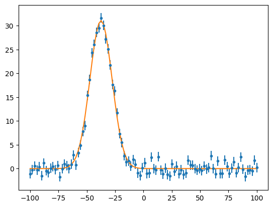
Plot the Data
>>> import matplotlib.pyplot as plt
>>> i = 32 # Chosen arbitrarily
>>> amp   = fit_data[i]['parameters']['amp']
>>> mu    = fit_data[i]['parameters']['mu']
>>> sigma = fit_data[i]['parameters']['sigma']
>>> plt.errorbar(x_data, y_data[:, i]['value'], yerr=y_data[:, i]['uncertainty'], fmt=".")
>>> plt.plot(x_data, amp * np.exp(-(x_data-mu)**2 / (2*sigma**2)))
>>> plt.show()